library(MOSuite)
#> Warning: replacing previous import 'S4Arrays::makeNindexFromArrayViewport' by
#> 'DelayedArray::makeNindexFromArrayViewport' when loading 'SummarizedExperiment'
Default plots from main functions
Default plots can be printed to the screen and/or saved to the disk.
# set options to print & save the plots
options(moo_print_plots = TRUE)
options(moo_save_plots = TRUE)
# when moo_save_plots is TRUE, plots are saved to this directory:
options(moo_plots_dir = "./figures")
See ?MOSuite::options for more information.
clean
moo <- create_multiOmicDataSet_from_dataframes(
  sample_metadata = as.data.frame(nidap_sample_metadata),
  counts_dat = as.data.frame(nidap_raw_counts)
) |>
  clean_raw_counts()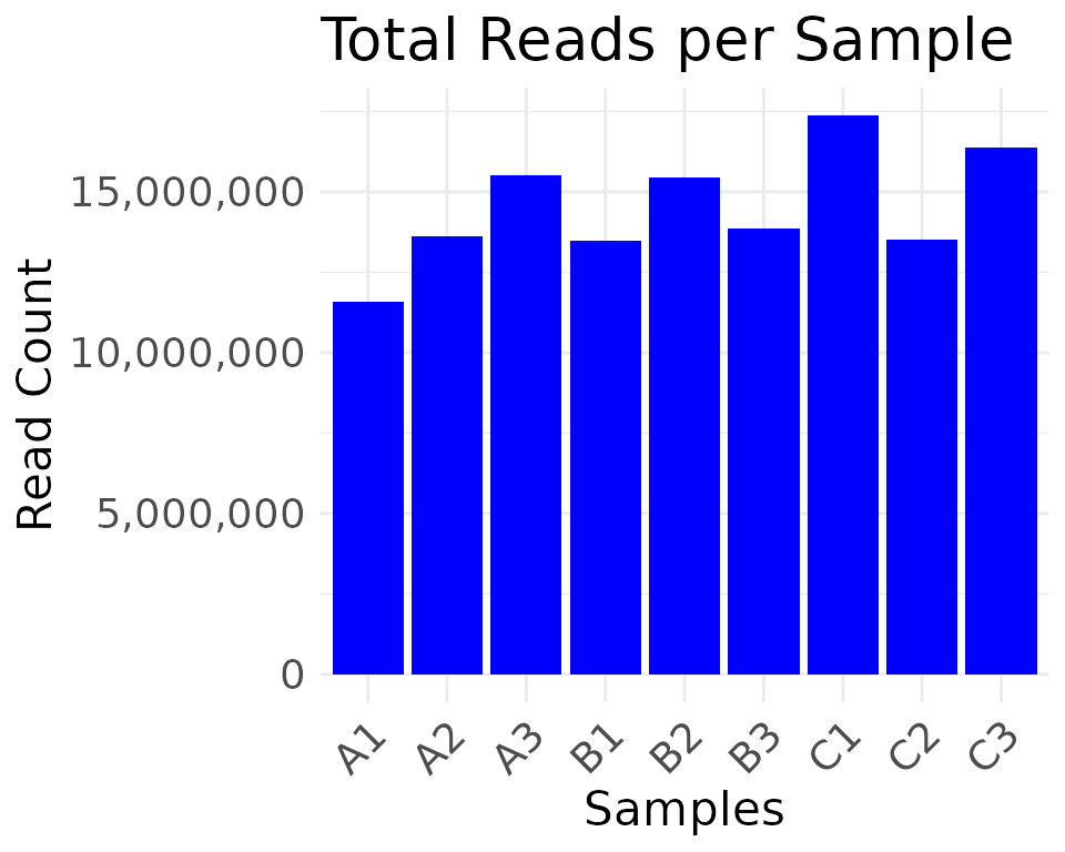
#> Saving 5 x 4 in image
#> * cleaning raw counts
#>
#> Not able to identify multiple id's in GeneName
#>
#> Columns that can be used to aggregate gene information GeneName
#>
#> Aggregating the counts for the same ID in different chromosome locations.
#> Column used to Aggregate duplicate IDs: GeneName
#> Number of rows before Collapse: 43280
#>
#> no duplicated IDs in GeneName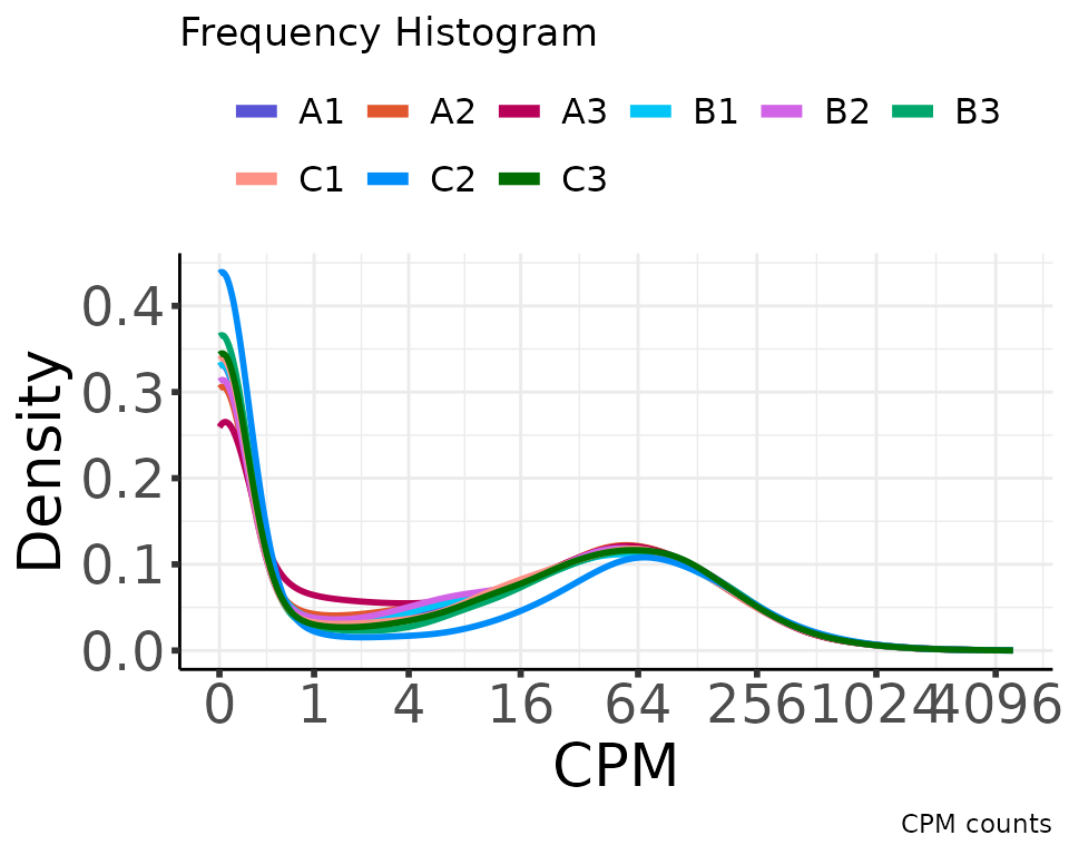
#> Saving 5 x 4 in imagefilter
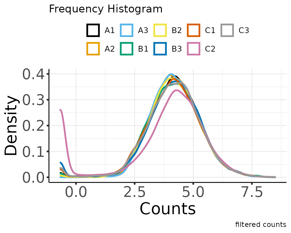
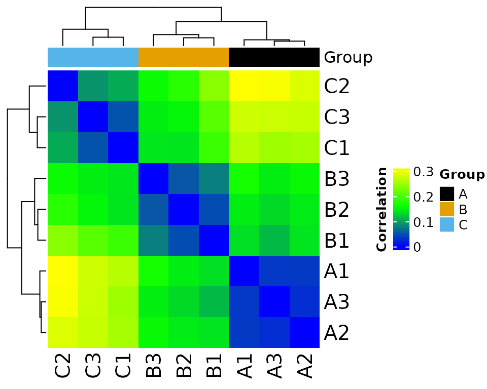
moo <- moo |>
  filter_counts(group_colname = "Group")
#> * filtering clean counts
#> Number of features after filtering: 7943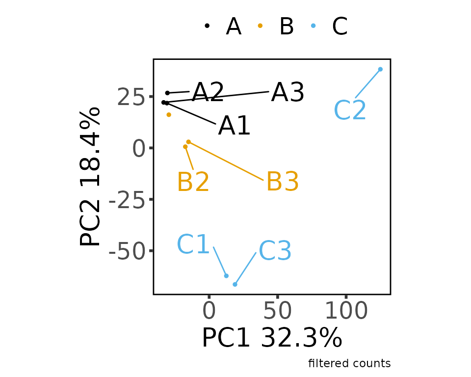
#> Saving 5 x 4 in imagenormalize
moo <- moo |>
  normalize_counts(group_colname = "Group")
#> * normalizing filt counts
#> Total number of features included: 7943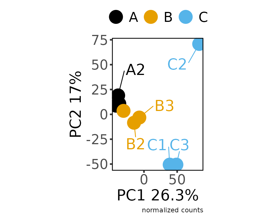
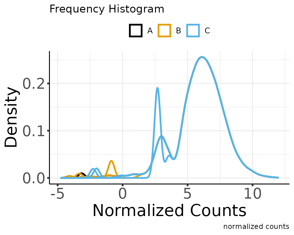
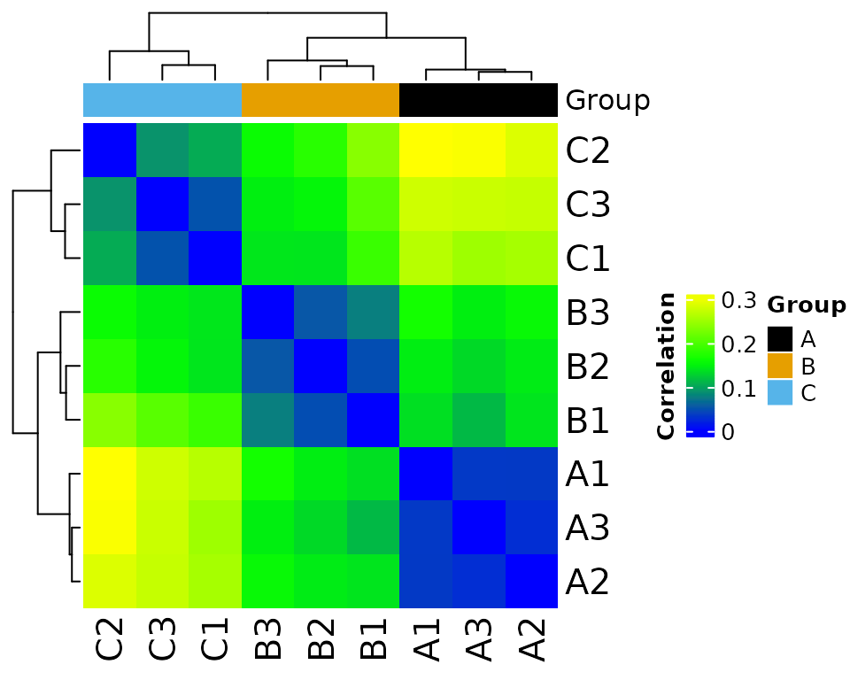
#> Saving 5 x 4 in image
#> Sample columns: A1, Sample columns: A2, Sample columns: A3, Sample columns: B1, Sample columns: B2, Sample columns: B3, Sample columns: C1, Sample columns: C2, Sample columns: C3
batch correct
moo <- moo |>
  batch_correct_counts(
    covariates_colname = "Group",
    batch_colname = "Batch",
    label_colname = "Label"
  )
#> * batch-correcting norm-voom counts
#> Found2batches
#> Adjusting for2covariate(s) or covariate level(s)
#> Standardizing Data across genes
#> Fitting L/S model and finding priors
#> Finding parametric adjustments
#> Adjusting the Data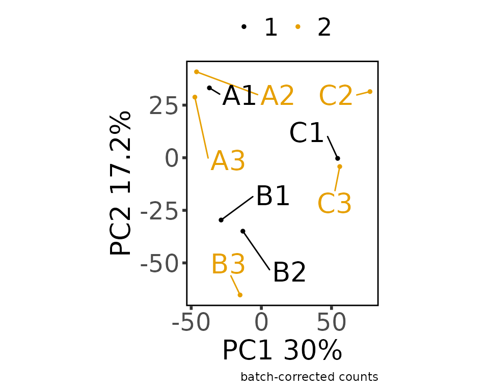
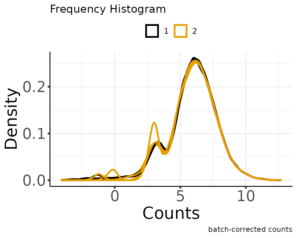
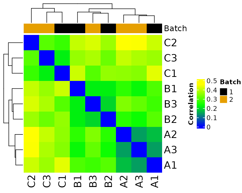
#> Saving 5 x 4 in image
#> The total number of features in output: 7943
#> Number of samples after batch correction: 10
differential expression
moo <- moo |>
  diff_counts(
    count_type = "filt",
    covariates_colnames = c("Group", "Batch"),
    contrast_colname = c("Group"),
    contrasts = c("B-A", "C-A", "B-C"),
    input_in_log_counts = FALSE,
    return_mean_and_sd = FALSE,
    voom_normalization_method = "quantile",
  )
#> * differential counts
#> Setting first column of `counts` as gene annotation.
#> Total number of genes included: 7943
#> `geom_smooth()` using method = 'gam' and formula = 'y ~ s(x, bs = "cs")'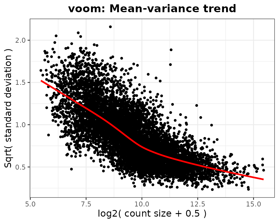
#> Saving 5 x 4 in image
#> `geom_smooth()` using method = 'gam' and formula = 'y ~ s(x, bs = "cs")'
filter differential features
moo <- moo |> filter_diff()
#> Joining with `by = join_by(GeneName)`
#> Joining with `by = join_by(GeneName)`
#> * filtering differential features
#> Total number of genes selected with adjpval < 0.05 and | logFC | > 1 is
#> sum(selgenes)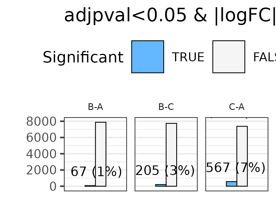
#> Saving 5 x 4 in imageSpecialized plots
3D PCA
plot_pca_3d(
  moo,
  count_type = "batch",
  principal_components = c(1, 2, 3),
  group_colname = "Group",
  label_colname = "Label"
)
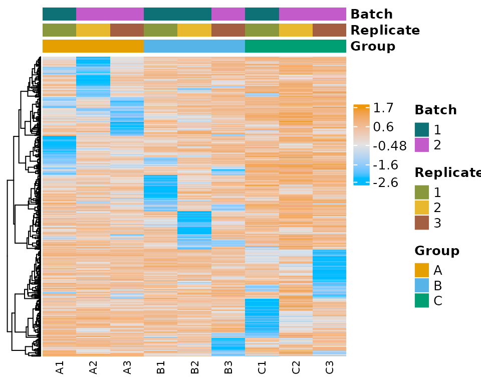
Expression Heatmap
heatmap_plot <- plot_expr_heatmap(
  moo,
  count_type = "norm",
  sub_count_type = "voom",
  group_colname = "Group"
)
#> The total number of genes in heatmap: 500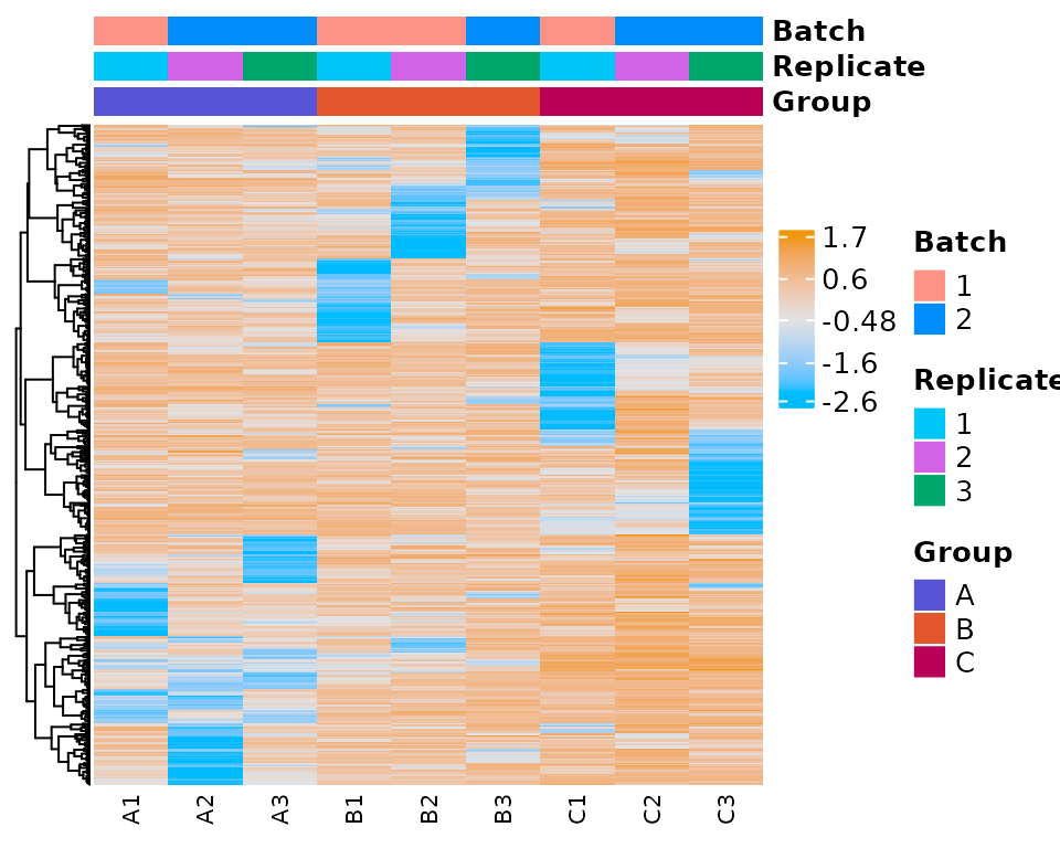
# print(heatmap_plot)Volcano
Enhanced
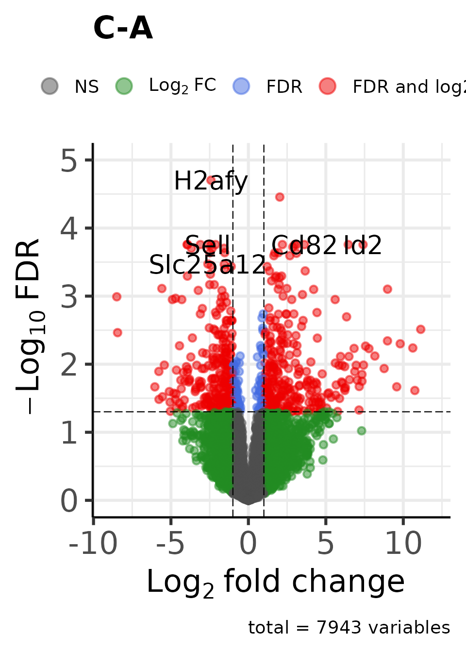
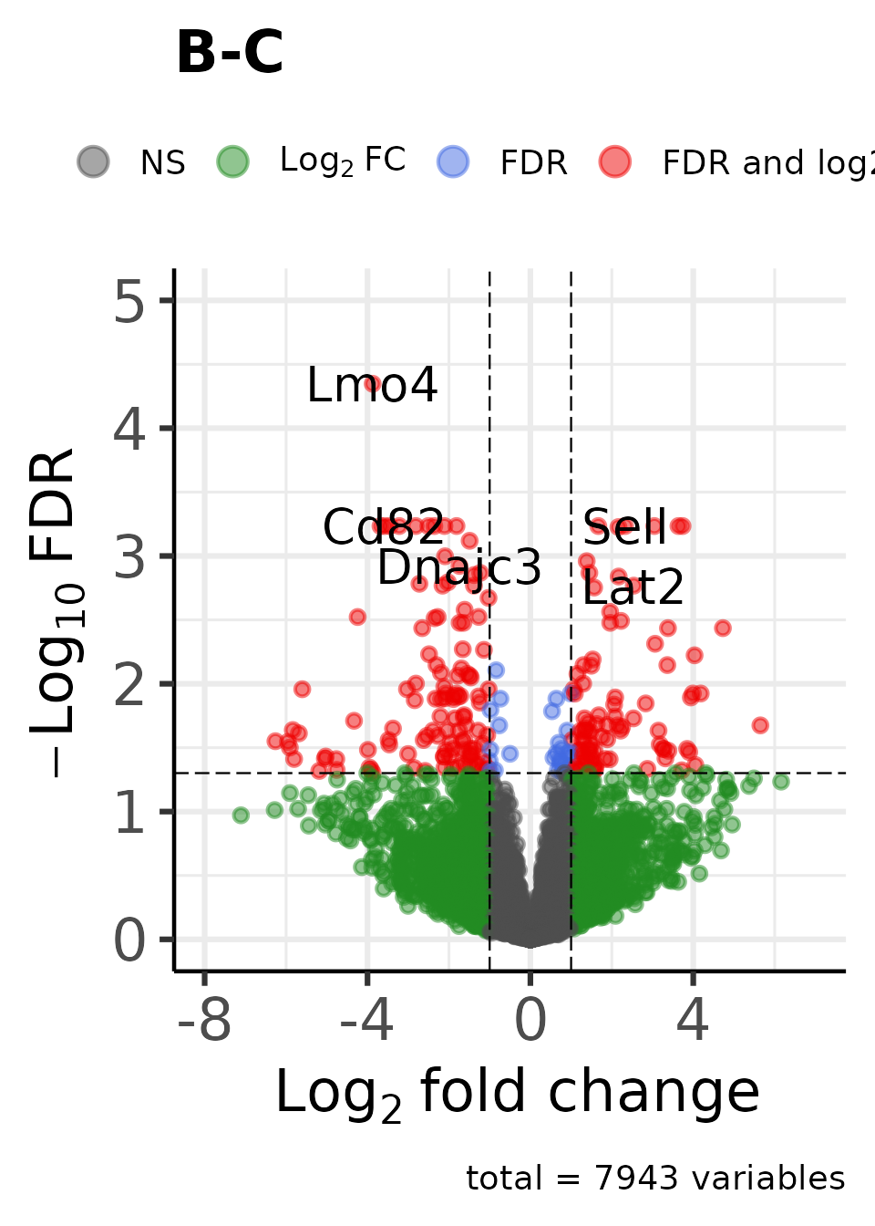
Create an enhanced volcano plot for each contrast:
dat_volcano_enhanced <- moo |>
  plot_volcano_enhanced()
#> Joining with `by = join_by(GeneName)`
#> Joining with `by = join_by(GeneName)`
#> Genes in initial dataset: 7943
#> Max y: 4.56088783571366
#> Warning: Using `size` aesthetic for lines was deprecated in ggplot2 3.4.0.
#> ℹ Please use `linewidth` instead.
#> ℹ The deprecated feature was likely used in the EnhancedVolcano package.
#>   Please report the issue to the authors.
#> This warning is displayed once per session.
#> Call `lifecycle::last_lifecycle_warnings()` to see where this warning was
#> generated.
#> Warning: The `size` argument of `element_line()` is deprecated as of ggplot2 3.4.0.
#> ℹ Please use the `linewidth` argument instead.
#> ℹ The deprecated feature was likely used in the EnhancedVolcano package.
#>   Please report the issue to the authors.
#> This warning is displayed once per session.
#> Call `lifecycle::last_lifecycle_warnings()` to see where this warning was
#> generated.
#> Genes in initial dataset: 7943
#>
#> Max y: 4.70280335204325
#>
#> Genes in initial dataset: 7943
#>
#> Max y: 4.34744066227962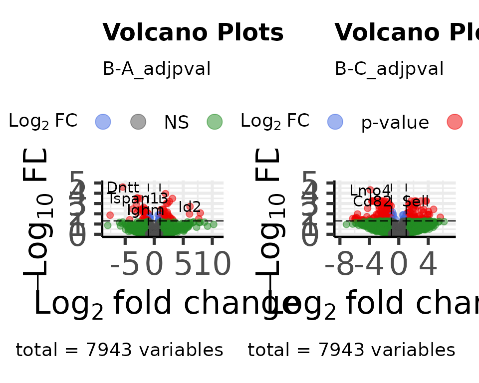
or plot only one contrast at a time by selecting the contrast from
the analyses slot:
dat_volcano_enhanced_B_A <- moo@analyses$diff[["B-A"]] |>
  plot_volcano_enhanced(
    feature_id_colname = "GeneName",
    change_colname = "logFC",
    signif_colname = "adjpval"
  )
#> Genes in initial dataset: 7943
#> Max y: 4.56088783571366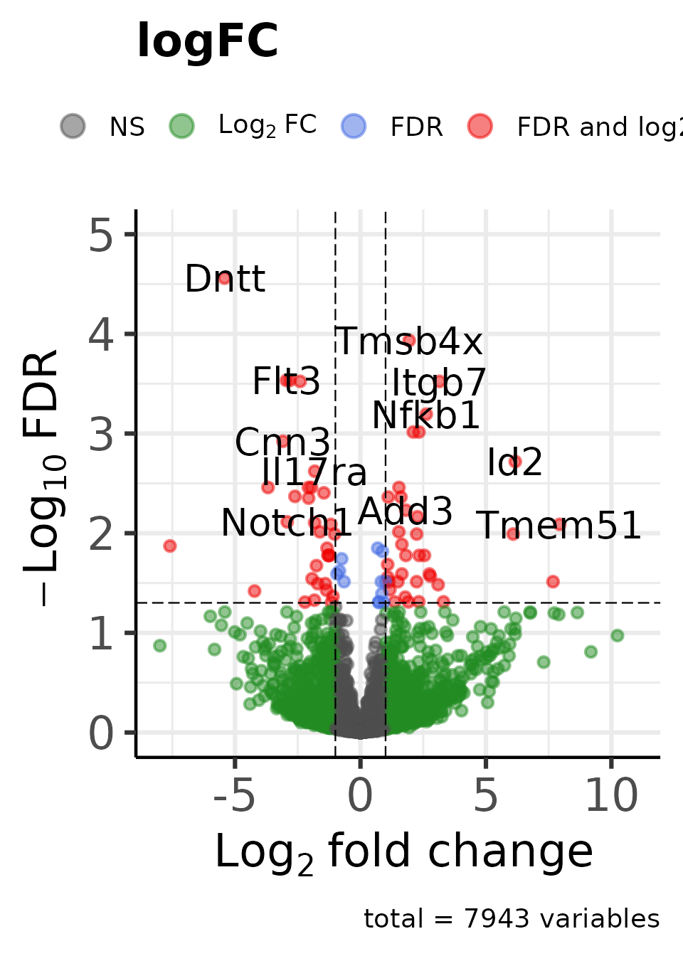
Summary
Create an enhanced volcano plot for each contrast and compose them in one figure:
dat_volcano_summary <- moo |>
  plot_volcano_summary()
#> Joining with `by = join_by(GeneName)`
#> Joining with `by = join_by(GeneName)`
#> Preparing table for contrast: B-A
#> Fold change column: B-A_logFC
#> Significance column: B-A_adjpval
#> Total number of features included in volcano plot: 7943
#> Preparing table for contrast: C-A
#> Fold change column: C-A_logFC
#> Significance column: C-A_adjpval
#> Total number of features included in volcano plot: 7943
#> Preparing table for contrast: B-C
#> Fold change column: B-C_logFC
#> Significance column: B-C_adjpval
#> Total number of features included in volcano plot: 7943
#> Running Enhanced Volcano:
#> Genes in initial dataset: 7943
#> Max y: 4.56088783571366
#> Genes in initial dataset: 7943
#> Max y: 4.70280335204325
#> Genes in initial dataset: 7943
#> Max y: 4.34744066227962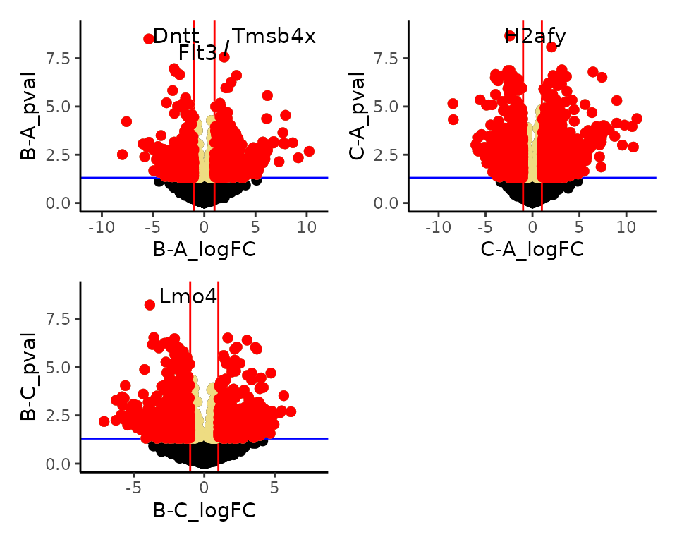
head(dat_volcano_summary)
#>       GeneName Contrast         FC     logFC     tstat         pval
#> B-A.1     Dntt      B-A -42.727551 -5.417095 -15.54572 3.460410e-09
#> B-A.2   Tmsb4x      B-A   3.845863  1.943307  12.82926 2.930649e-08
#> B-A.3     Flt3      B-A  -7.743692 -2.953022 -11.29797 1.173487e-07
#> B-A.4  Tspan13      B-A  -7.035795 -2.814713 -11.06018 1.476477e-07
#> B-A.5    Tapt1      B-A  -5.297586 -2.405335 -10.64544 2.226279e-07
#> B-A.6    Itgb7      B-A   8.882141  3.150907  10.62882 2.263833e-07
#>            adjpval
#> B-A.1 2.748604e-05
#> B-A.2 1.163907e-04
#> B-A.3 2.931915e-04
#> B-A.4 2.931915e-04
#> B-A.5 2.996937e-04
#> B-A.6 2.996937e-04
Venn Diagram
venn_dat <- dat_volcano_summary |> plot_venn_diagram()
#> All intersections: 1:7,c(1, 2, 3, 4, 5, 6, 7),c(6, 19, 36, 136, 6, 42, 396),c("Yes", "Yes", "Yes", "Yes", "Yes", "Yes", "Yes")
#> Intersections returned: 1:7,c(1, 2, 3, 4, 5, 6, 7),c(6, 19, 36, 136, 6, 42, 396)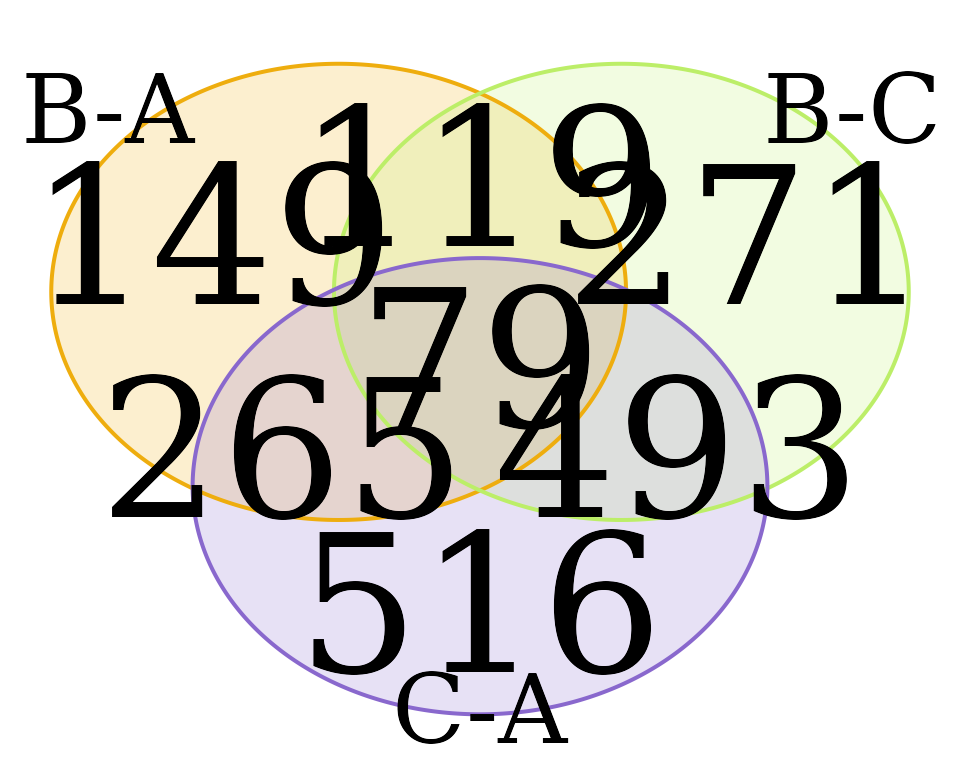
head(venn_dat)
#>    Gene      Intersection Id Size
#> 1   Id2 (B-A ∩ B-C ∩ C-A)  1    6
#> 2   Myc (B-A ∩ B-C ∩ C-A)  1    6
#> 3 Prr13 (B-A ∩ B-C ∩ C-A)  1    6
#> 4  Cd34 (B-A ∩ B-C ∩ C-A)  1    6
#> 5 Esyt1 (B-A ∩ B-C ∩ C-A)  1    6
#> 6 Mgat1 (B-A ∩ B-C ∩ C-A)  1    6
Customizing plots
Plots from main functions
You can create the plots generated by the main analysis functions directly so you can customize them to fit your needs.
See the visualization reference for a full list of plotting functions.
Examples
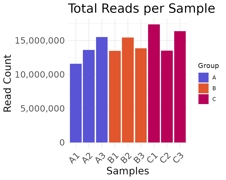
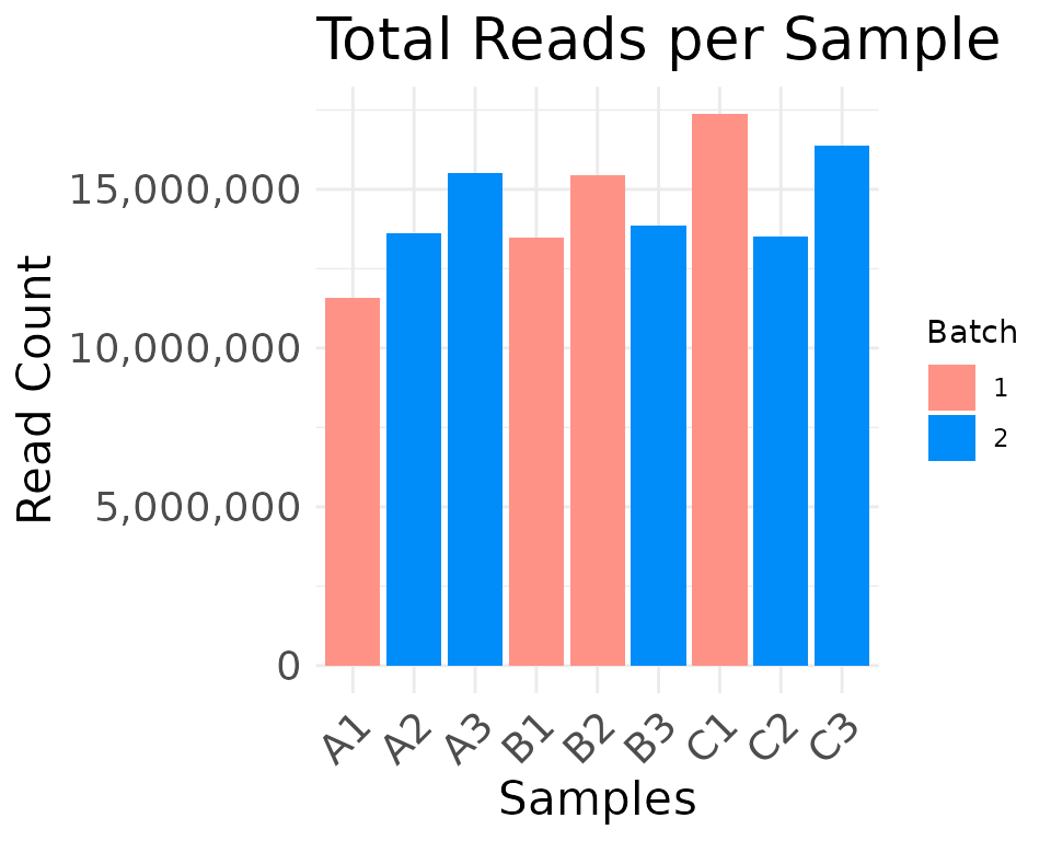
Plot the read depth of the clean counts, using either the
Group column or the Batch column from the
metadata for the fill colors:
plot_read_depth(
  moo,
  count_type = "clean",
  group_colname = "Group"
)
plot_read_depth(
  moo,
  count_type = "clean",
  group_colname = "Batch"
)
Customizing ggplot objects
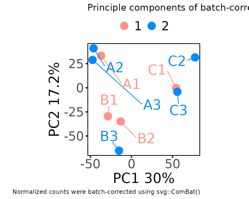
Plotting functions that use ggplot2 return ggplot objects. You can customize them by adding more ggplot layers, just like any other ggplot.
plot_pca_2d(
  moo,
  count_type = "batch",
  principal_components = c(1, 2),
  group_colname = "Batch",
  label_colname = "Label"
) +
  ggplot2::labs(
    title = "Principle components of batch-corrected counts",
    caption = "Normalized counts were batch-corrected using svg::ComBat()"
  )
Custom colors
MOSuite comes bundled with a default palette:

When creating a multiOmicDataSet object such as with
create_multiOmicDataSet_from_dataframes(), default colors
are automatically picked from mosuite_palette and set in
the analyses slot. You can access the defaults directly:
moo@analyses$colors
#> $Sample
#>        A1        A2        A3        B1        B2        B3        C1        C2
#> "#5954d6" "#e1562c" "#b80058" "#00c6f8" "#d163e6" "#00a76c" "#ff9287" "#008cf9"
#>        C3
#> "#006e00"
#>
#> $Group
#>         A         B         C
#> "#5954d6" "#e1562c" "#b80058"
#>
#> $Replicate
#>         1         2         3
#> "#00c6f8" "#d163e6" "#00a76c"
#>
#> $Batch
#>         1         2
#> "#ff9287" "#008cf9"
#>
#> $Label
#>        A1        A2        A3        B1        B2        B3        C1        C2
#> "#5954d6" "#e1562c" "#b80058" "#00c6f8" "#d163e6" "#00a76c" "#ff9287" "#008cf9"
#>        C3
#> "#006e00"
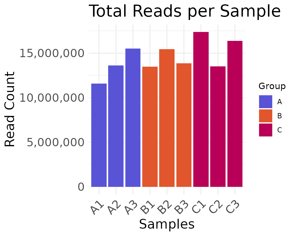
The plotting functions access these colors by default, unless
overridden with the color_values argument:
# color palette accessed from moo@analyses$colors[['Group']]
plot_read_depth(
  moo,
  count_type = "clean",
  group_colname = "Group"
)
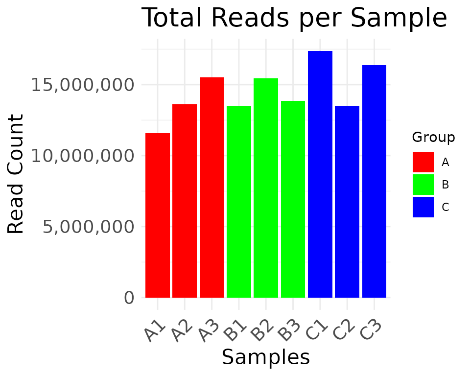
# color palette overridden by color_values
plot_read_depth(
  moo,
  count_type = "clean",
  group_colname = "Group",
  color_values = c(A = "red", B = "green", C = "blue")
)
You can change the default colors in the multiOmicDataSet so that all plotting functions will use your chosen color palette.
moo@analyses$colors[["Batch"]] <- c("1" = "#0E7175", "2" = "#C35BCA")
moo@analyses$colors[["Replicate"]] <- c(
  "1" = "#89973D",
  "2" = "#E8B92F",
  "3" = "#A45E41"
)
moo@analyses$colors[["Group"]] <- c(A = "#E69F00", B = "#56B4E9", C = "#009E73")
View the colors in a multiOmicDataSet with
display_colors():
display_colors(moo)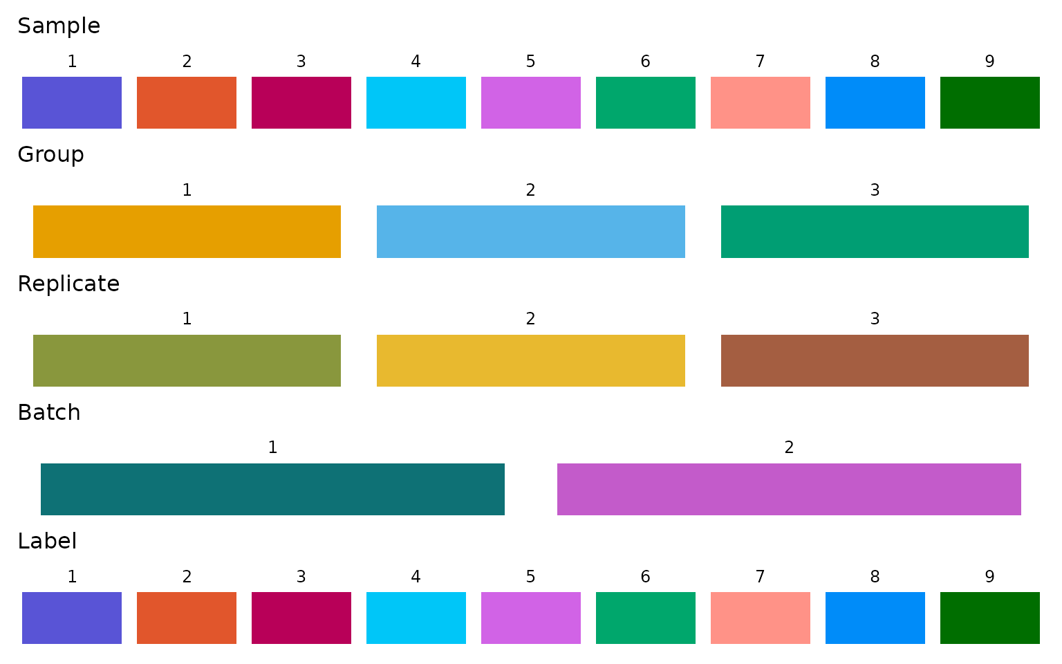
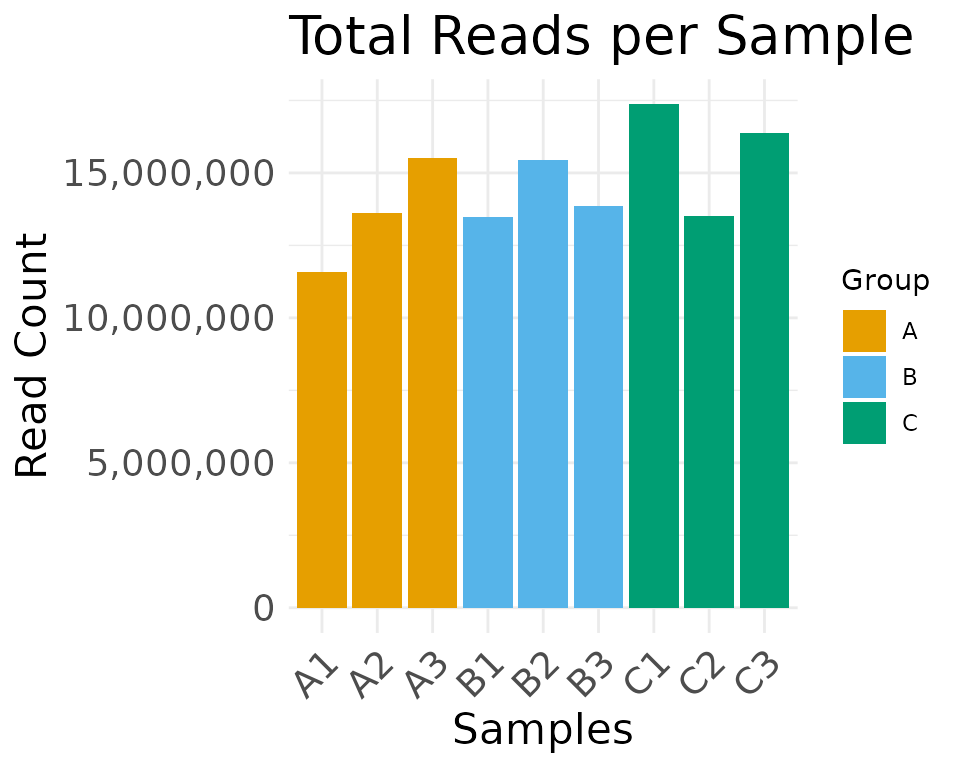
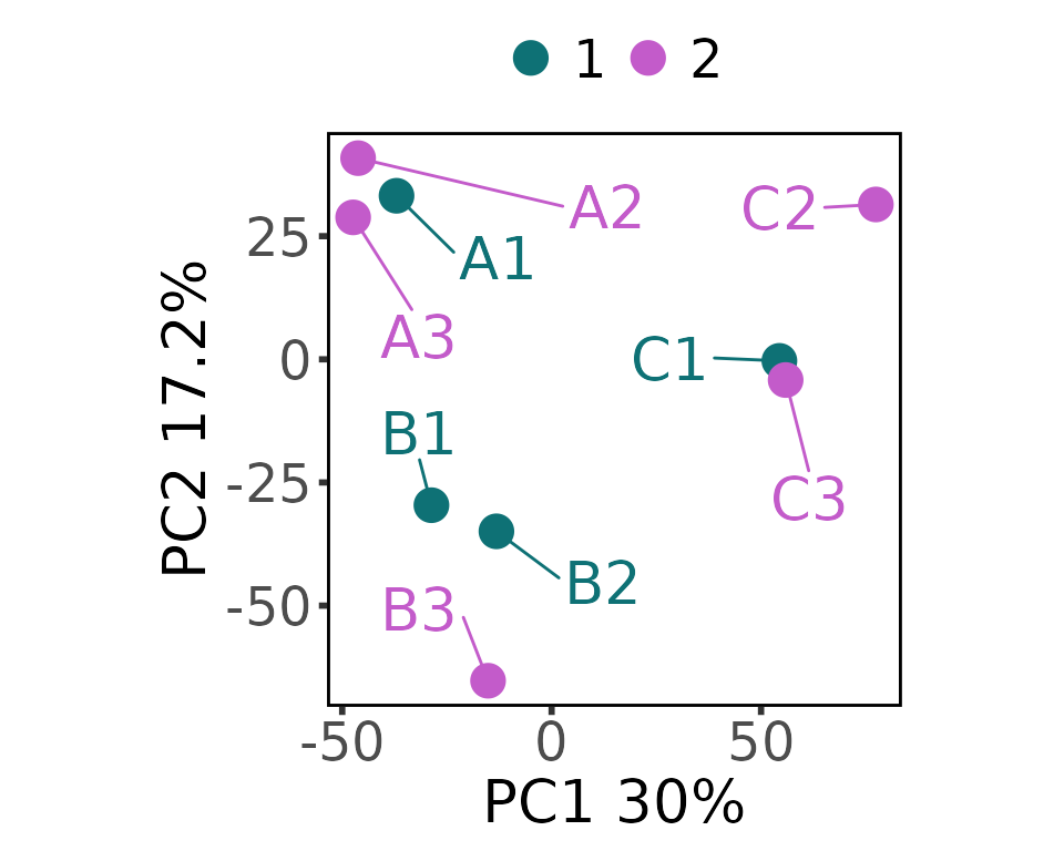
Plotting functions will then use the custom colors set in
moo@analyses$colors:
plot_read_depth(
  moo,
  count_type = "clean",
  group_colname = "Group"
)
plot_pca_2d(
  moo,
  count_type = "batch",
  group_colname = "Batch"
)
plot_expr_heatmap(
  moo,
  count_type = "norm",
  sub_count_type = "voom",
  group_colname = "Group"
)
#> The total number of genes in heatmap: 500